
Algebra computacional con Sympy#
Basado en Taming math and physics using SymPy y Sympy : Symbolic Mathematics in Python
Conceptos básicos de Sympy#
# Importar librerias de cálculo matemático
from sympy import *
import numpy as np

# Importar libreria para gráficos
import matplotlib.pyplot as plt
%matplotlib inline
# Forzar una expresión como simbólica
expr = S("1/7")
print ("Tipo expresión: ", expr, type(expr))

# Obtener su valor numérico
num = N("1/7")
print ("Tipo numérico: ", num, type(num))

# Operaciones para Racional y Flotante de sympy
print (expr+1)
print (num+1)
Tipo expresión:  1/7 <class 'sympy.core.numbers.Rational'>
Tipo numérico:  0.142857142857143 <class 'sympy.core.numbers.Float'>
8/7
1.14285714285714
# Cadena de texto sencilla
x='1/7'
print(type(x))

# Expresión simbólica de Sympy, usando comando S("expresion")
y=S('1/7')
print(type(y))
<class 'str'>
<class 'sympy.core.numbers.Rational'>
# Ejemplos de expresiones y operaciones con las mismas
## Como racional
print(S('1/7'))

## Como numérico
print(N('1/7'))

## Operación como racional
print(S('1/7')+1)

## Operación como numérico
print(N('1/7')+1)

## Tipos racional y flotante
print(type(S('1/7')),type(N('1/7')))
1/7
0.142857142857143
8/7
1.14285714285714
<class 'sympy.core.numbers.Rational'> <class 'sympy.core.numbers.Float'>
# pi es la expresión de Sympy, mientras que np.pi es la de Numpy

print (pi, "\t", type(pi))
print (pi + 1, "\t", type(pi+1))
print (N(pi+1), "\t", type(N(pi+1)))
print (np.pi, "\t", type(np.pi))
print (np.pi+1, "\t", type(np.pi+1))
pi 	 <class 'sympy.core.numbers.Pi'>
1 + pi 	 <class 'sympy.core.add.Add'>
4.14159265358979 	 <class 'sympy.core.numbers.Float'>
3.141592653589793 	 <class 'float'>
4.141592653589793 	 <class 'float'>
# Poniendo a Sympy a que imprima resultados bonitos
init_printing(use_latex=True)
pi, expr

# Poniendo a Sympy a que imprima resultados NO bonitos
init_printing(use_latex=False)
pi, expr
(π, 1/7)
Expresiones#
# Usando variables regulares de Python
t=2
y=3*t
y
6
# Tiene el tag: raises-exception, para que aunque tiene error continue compilando el notebook (View,Cell Toolbar,Tags)

# Usando variables simbólicas sin Sympy

expr = 2*x + 3*x - sin(x) - 3*x + 42
---------------------------------------------------------------------------
TypeError                                 Traceback (most recent call last)
<ipython-input-47-519f78f4039f> in <module>
      3 # Usando variables simbólicas sin Sympy
      4
----> 5 expr = 2*x + 3*x - sin(x) - 3*x + 42

TypeError: unsupported operand type(s) for -: 'str' and 'sin'
Definir variables#
# Definir variables simbólicas con Sympy

## Definir las variables
x,y,z  = symbols("x y z")

## Ahora sí, escribir la expresión
expr = 2*x + 3*x - sin(x) - 3*x + 42
expr
2⋅x - sin(x) + 42
nu,mu = symbols("n,m")
nu*2+mu
m + 2⋅n
g,a = symbols("\\gamma \\alpha")
g*2+a
\alpha + 2⋅\gamma
r, p, t = symbols("r, \\phi, \\theta")
2*r+3*p+5*t
3⋅\phi + 5⋅\theta + 2⋅r
## Revisión de tipos luego de Definir las variables x,y,z

w=3
print(type(w))
print(type(x))
<class 'int'>
<class 'sympy.core.symbol.Symbol'>
# Poniendo a Sympy a que imprima resultados bonitos, de esta celda en adelante

init_printing(use_latex=True)
Expandir y factorizar#
# Expandir

expand( (x+3)**2 )

# Factorizar

factor( x**2 + 5*x + 6 )

Sustituciones#
# Definir la expresión

expr = (sin(x) + cos(y)) / 2
expr

# Sustituir "x" por 1, e "y" por 2

expr.subs({x: 1, y:2})

# Obtener el valor numérico flotante

N(expr.subs({x: 1, y:2}))

# Sustituir "x" por otra expresión

expr.subs({x: y**2+1})

# Sustituir por otra expresión, y la única variable "y", sustituirla por el número 2

expr.subs({x: y**2+1}).subs({y: 2})

# Obtener el valor numérico flotante, dos opciones

print(N(expr.subs({x: y**2+1}).subs({y: 2})))
print(expr.subs({x: y**2+1}).subs({y: 2}).n())
-0.687535555605140
-0.687535555605140
Prueba de igualdad#
# Definimos algunas expresiones

p = (x-5)*(x+5)
q = x**2 - 25
z = (x**2-9)/(x-3)
w = x+3
# No se puede comparar directamente usando el ==

print(p == q)
print(p - q == 0 )
False
False
print(z == w)
print(z - w == 0 )
False
False
simplify(z)

# Ejemplo 1

print(simplify(p - q))
print(simplify(p - q) == 0)
0
True
# Ejemplo 2

print(simplify(z))
print(simplify(z)==w)
x + 3
True
# Ejemplo 3

expr1 = (x**2-9)/(x-3)
expr2 = (x+3)

expr1.equals(expr2)
True
# Verificación del ejemplo 3

simplify(expr1)
Solucionadores#
# Encontrar el valor de X
solve(5*x-10)

# Encontrar el valor de y
solve(5*x-x**2-y,y)

# Encontrar valores de x
s=solve(x**2 + 5*x +6)
s[0],s[1]

# Tipo para lista y los elementos
type(s),type(s[0])
(list, sympy.core.numbers.Integer)
# Encontrar valores de x y mostrarlos
solve(x**2+5*x+6)

# Encontrar valores de x y mostrarlos además del tipo de datos
sol = solve( x**2 + 2*x - 8, x)
sol[0], sol[1], type(sol[0]), type(sol[1])
(-4, 2, sympy.core.numbers.Integer, sympy.core.numbers.Integer)
# Generar una expresión usando un valor de la solución
sol[0]+x

# Al agregarse un flotante a la suma se vuelve flotante el resultado
print(sol[0]+1.)
type(sol[0]+1.)
-3.00000000000000
sympy.core.numbers.Float
# Encontrando las famosas raices de la ecuación cuadrática
a, b, c = symbols('a b c')
solve( a*x**2 + b*x + c, x)

# Encontrando sólo una de las raices la ecuación cuadrática
sol = solve( a*x**2 + b*x + c, x)[0]
sol

# Substituyento por valores y obteniendo una raiz o número complejo
sol.subs({a:1, b:2, c:3})

# Substituyento por valores y obteniendo un número real
sol.subs({a:1, b:5, c:6})

Completar el cuadrado de modo que: \(x^2-4x+7=(x-h)^2+k\) para algunas constantes \(h\) y \(k\).
Resolvemos \((x-h)^2+k-(x^2-4x+7)=0\)
# Resolver
h, k = symbols('h k')

# Encontrar valores de "h" y de "k"
solve( (x-h)**2 + k - (x**2-4*x+7), [h,k] )

# Verificar que efectivamente h==2 y que k==3
((x-2)**2 + 3).expand()

Solucionar el sistema de ecuaciones:
# Se resuelve indicandole las dos ecuaciones
solve([x**2+y, 3*y-x])

# Otro ejemplo de un sistema de ecuaciones
print(solve([x+y-6, x-y-2]))
{x: 4, y: 2}
# Ejemplo de solución de una inecuación
print(solve(x-2>3))
(5 < x) & (x < oo)
# Explorar más a profundidad la documentación
help (solve)
Help on function solve in module sympy.solvers.solvers:

solve(f, *symbols, **flags)
    Algebraically solves equations and systems of equations.

    Explanation
    ===========

    Currently supported:
        - polynomial
        - transcendental
        - piecewise combinations of the above
        - systems of linear and polynomial equations
        - systems containing relational expressions

    Examples
    ========

    The output varies according to the input and can be seen by example:

        >>> from sympy import solve, Poly, Eq, Function, exp
        >>> from sympy.abc import x, y, z, a, b
        >>> f = Function('f')

    Boolean or univariate Relational:

        >>> solve(x < 3)
        (-oo < x) & (x < 3)


    To always get a list of solution mappings, use flag dict=True:

        >>> solve(x - 3, dict=True)
        [{x: 3}]
        >>> sol = solve([x - 3, y - 1], dict=True)
        >>> sol
        [{x: 3, y: 1}]
        >>> sol[0][x]
        3
        >>> sol[0][y]
        1


    To get a list of *symbols* and set of solution(s) use flag set=True:

        >>> solve([x**2 - 3, y - 1], set=True)
        ([x, y], {(-sqrt(3), 1), (sqrt(3), 1)})


    Single expression and single symbol that is in the expression:

        >>> solve(x - y, x)
        [y]
        >>> solve(x - 3, x)
        [3]
        >>> solve(Eq(x, 3), x)
        [3]
        >>> solve(Poly(x - 3), x)
        [3]
        >>> solve(x**2 - y**2, x, set=True)
        ([x], {(-y,), (y,)})
        >>> solve(x**4 - 1, x, set=True)
        ([x], {(-1,), (1,), (-I,), (I,)})

    Single expression with no symbol that is in the expression:

        >>> solve(3, x)
        []
        >>> solve(x - 3, y)
        []

    Single expression with no symbol given. In this case, all free *symbols*
    will be selected as potential *symbols* to solve for. If the equation is
    univariate then a list of solutions is returned; otherwise - as is the case
    when *symbols* are given as an iterable of length greater than 1 - a list of
    mappings will be returned:

        >>> solve(x - 3)
        [3]
        >>> solve(x**2 - y**2)
        [{x: -y}, {x: y}]
        >>> solve(z**2*x**2 - z**2*y**2)
        [{x: -y}, {x: y}, {z: 0}]
        >>> solve(z**2*x - z**2*y**2)
        [{x: y**2}, {z: 0}]

    When an object other than a Symbol is given as a symbol, it is
    isolated algebraically and an implicit solution may be obtained.
    This is mostly provided as a convenience to save you from replacing
    the object with a Symbol and solving for that Symbol. It will only
    work if the specified object can be replaced with a Symbol using the
    subs method:

    >>> solve(f(x) - x, f(x))
    [x]
    >>> solve(f(x).diff(x) - f(x) - x, f(x).diff(x))
    [x + f(x)]
    >>> solve(f(x).diff(x) - f(x) - x, f(x))
    [-x + Derivative(f(x), x)]
    >>> solve(x + exp(x)**2, exp(x), set=True)
    ([exp(x)], {(-sqrt(-x),), (sqrt(-x),)})

    >>> from sympy import Indexed, IndexedBase, Tuple, sqrt
    >>> A = IndexedBase('A')
    >>> eqs = Tuple(A[1] + A[2] - 3, A[1] - A[2] + 1)
    >>> solve(eqs, eqs.atoms(Indexed))
    {A[1]: 1, A[2]: 2}

        * To solve for a symbol implicitly, use implicit=True:

            >>> solve(x + exp(x), x)
            [-LambertW(1)]
            >>> solve(x + exp(x), x, implicit=True)
            [-exp(x)]

        * It is possible to solve for anything that can be targeted with
          subs:

            >>> solve(x + 2 + sqrt(3), x + 2)
            [-sqrt(3)]
            >>> solve((x + 2 + sqrt(3), x + 4 + y), y, x + 2)
            {y: -2 + sqrt(3), x + 2: -sqrt(3)}

        * Nothing heroic is done in this implicit solving so you may end up
          with a symbol still in the solution:

            >>> eqs = (x*y + 3*y + sqrt(3), x + 4 + y)
            >>> solve(eqs, y, x + 2)
            {y: -sqrt(3)/(x + 3), x + 2: -2*x/(x + 3) - 6/(x + 3) + sqrt(3)/(x + 3)}
            >>> solve(eqs, y*x, x)
            {x: -y - 4, x*y: -3*y - sqrt(3)}

        * If you attempt to solve for a number remember that the number
          you have obtained does not necessarily mean that the value is
          equivalent to the expression obtained:

            >>> solve(sqrt(2) - 1, 1)
            [sqrt(2)]
            >>> solve(x - y + 1, 1)  # /!\ -1 is targeted, too
            [x/(y - 1)]
            >>> [_.subs(z, -1) for _ in solve((x - y + 1).subs(-1, z), 1)]
            [-x + y]

        * To solve for a function within a derivative, use ``dsolve``.

    Single expression and more than one symbol:

        * When there is a linear solution:

            >>> solve(x - y**2, x, y)
            [(y**2, y)]
            >>> solve(x**2 - y, x, y)
            [(x, x**2)]
            >>> solve(x**2 - y, x, y, dict=True)
            [{y: x**2}]

        * When undetermined coefficients are identified:

            * That are linear:

                >>> solve((a + b)*x - b + 2, a, b)
                {a: -2, b: 2}

            * That are nonlinear:

                >>> solve((a + b)*x - b**2 + 2, a, b, set=True)
                ([a, b], {(-sqrt(2), sqrt(2)), (sqrt(2), -sqrt(2))})

        * If there is no linear solution, then the first successful
          attempt for a nonlinear solution will be returned:

            >>> solve(x**2 - y**2, x, y, dict=True)
            [{x: -y}, {x: y}]
            >>> solve(x**2 - y**2/exp(x), x, y, dict=True)
            [{x: 2*LambertW(-y/2)}, {x: 2*LambertW(y/2)}]
            >>> solve(x**2 - y**2/exp(x), y, x)
            [(-x*sqrt(exp(x)), x), (x*sqrt(exp(x)), x)]

    Iterable of one or more of the above:

        * Involving relationals or bools:

            >>> solve([x < 3, x - 2])
            Eq(x, 2)
            >>> solve([x > 3, x - 2])
            False

        * When the system is linear:

            * With a solution:

                >>> solve([x - 3], x)
                {x: 3}
                >>> solve((x + 5*y - 2, -3*x + 6*y - 15), x, y)
                {x: -3, y: 1}
                >>> solve((x + 5*y - 2, -3*x + 6*y - 15), x, y, z)
                {x: -3, y: 1}
                >>> solve((x + 5*y - 2, -3*x + 6*y - z), z, x, y)
                {x: 2 - 5*y, z: 21*y - 6}

            * Without a solution:

                >>> solve([x + 3, x - 3])
                []

        * When the system is not linear:

            >>> solve([x**2 + y -2, y**2 - 4], x, y, set=True)
            ([x, y], {(-2, -2), (0, 2), (2, -2)})

        * If no *symbols* are given, all free *symbols* will be selected and a
          list of mappings returned:

            >>> solve([x - 2, x**2 + y])
            [{x: 2, y: -4}]
            >>> solve([x - 2, x**2 + f(x)], {f(x), x})
            [{x: 2, f(x): -4}]

        * If any equation does not depend on the symbol(s) given, it will be
          eliminated from the equation set and an answer may be given
          implicitly in terms of variables that were not of interest:

            >>> solve([x - y, y - 3], x)
            {x: y}

    **Additional Examples**

    ``solve()`` with check=True (default) will run through the symbol tags to
    elimate unwanted solutions. If no assumptions are included, all possible
    solutions will be returned:

        >>> from sympy import Symbol, solve
        >>> x = Symbol("x")
        >>> solve(x**2 - 1)
        [-1, 1]

    By using the positive tag, only one solution will be returned:

        >>> pos = Symbol("pos", positive=True)
        >>> solve(pos**2 - 1)
        [1]

    Assumptions are not checked when ``solve()`` input involves
    relationals or bools.

    When the solutions are checked, those that make any denominator zero
    are automatically excluded. If you do not want to exclude such solutions,
    then use the check=False option:

        >>> from sympy import sin, limit
        >>> solve(sin(x)/x)  # 0 is excluded
        [pi]

    If check=False, then a solution to the numerator being zero is found: x = 0.
    In this case, this is a spurious solution since $\sin(x)/x$ has the well
    known limit (without dicontinuity) of 1 at x = 0:

        >>> solve(sin(x)/x, check=False)
        [0, pi]

    In the following case, however, the limit exists and is equal to the
    value of x = 0 that is excluded when check=True:

        >>> eq = x**2*(1/x - z**2/x)
        >>> solve(eq, x)
        []
        >>> solve(eq, x, check=False)
        [0]
        >>> limit(eq, x, 0, '-')
        0
        >>> limit(eq, x, 0, '+')
        0

    **Disabling High-Order Explicit Solutions**

    When solving polynomial expressions, you might not want explicit solutions
    (which can be quite long). If the expression is univariate, ``CRootOf``
    instances will be returned instead:

        >>> solve(x**3 - x + 1)
        [-1/((-1/2 - sqrt(3)*I/2)*(3*sqrt(69)/2 + 27/2)**(1/3)) - (-1/2 -
        sqrt(3)*I/2)*(3*sqrt(69)/2 + 27/2)**(1/3)/3, -(-1/2 +
        sqrt(3)*I/2)*(3*sqrt(69)/2 + 27/2)**(1/3)/3 - 1/((-1/2 +
        sqrt(3)*I/2)*(3*sqrt(69)/2 + 27/2)**(1/3)), -(3*sqrt(69)/2 +
        27/2)**(1/3)/3 - 1/(3*sqrt(69)/2 + 27/2)**(1/3)]
        >>> solve(x**3 - x + 1, cubics=False)
        [CRootOf(x**3 - x + 1, 0),
         CRootOf(x**3 - x + 1, 1),
         CRootOf(x**3 - x + 1, 2)]

    If the expression is multivariate, no solution might be returned:

        >>> solve(x**3 - x + a, x, cubics=False)
        []

    Sometimes solutions will be obtained even when a flag is False because the
    expression could be factored. In the following example, the equation can
    be factored as the product of a linear and a quadratic factor so explicit
    solutions (which did not require solving a cubic expression) are obtained:

        >>> eq = x**3 + 3*x**2 + x - 1
        >>> solve(eq, cubics=False)
        [-1, -1 + sqrt(2), -sqrt(2) - 1]

    **Solving Equations Involving Radicals**

    Because of SymPy's use of the principle root, some solutions
    to radical equations will be missed unless check=False:

        >>> from sympy import root
        >>> eq = root(x**3 - 3*x**2, 3) + 1 - x
        >>> solve(eq)
        []
        >>> solve(eq, check=False)
        [1/3]

    In the above example, there is only a single solution to the
    equation. Other expressions will yield spurious roots which
    must be checked manually; roots which give a negative argument
    to odd-powered radicals will also need special checking:

        >>> from sympy import real_root, S
        >>> eq = root(x, 3) - root(x, 5) + S(1)/7
        >>> solve(eq)  # this gives 2 solutions but misses a 3rd
        [CRootOf(7*x**5 - 7*x**3 + 1, 1)**15,
        CRootOf(7*x**5 - 7*x**3 + 1, 2)**15]
        >>> sol = solve(eq, check=False)
        >>> [abs(eq.subs(x,i).n(2)) for i in sol]
        [0.48, 0.e-110, 0.e-110, 0.052, 0.052]

    The first solution is negative so ``real_root`` must be used to see that it
    satisfies the expression:

        >>> abs(real_root(eq.subs(x, sol[0])).n(2))
        0.e-110

    If the roots of the equation are not real then more care will be
    necessary to find the roots, especially for higher order equations.
    Consider the following expression:

        >>> expr = root(x, 3) - root(x, 5)

    We will construct a known value for this expression at x = 3 by selecting
    the 1-th root for each radical:

        >>> expr1 = root(x, 3, 1) - root(x, 5, 1)
        >>> v = expr1.subs(x, -3)

    The ``solve`` function is unable to find any exact roots to this equation:

        >>> eq = Eq(expr, v); eq1 = Eq(expr1, v)
        >>> solve(eq, check=False), solve(eq1, check=False)
        ([], [])

    The function ``unrad``, however, can be used to get a form of the equation
    for which numerical roots can be found:

        >>> from sympy.solvers.solvers import unrad
        >>> from sympy import nroots
        >>> e, (p, cov) = unrad(eq)
        >>> pvals = nroots(e)
        >>> inversion = solve(cov, x)[0]
        >>> xvals = [inversion.subs(p, i) for i in pvals]

    Although ``eq`` or ``eq1`` could have been used to find ``xvals``, the
    solution can only be verified with ``expr1``:

        >>> z = expr - v
        >>> [xi.n(chop=1e-9) for xi in xvals if abs(z.subs(x, xi).n()) < 1e-9]
        []
        >>> z1 = expr1 - v
        >>> [xi.n(chop=1e-9) for xi in xvals if abs(z1.subs(x, xi).n()) < 1e-9]
        [-3.0]

    Parameters
    ==========

    f :
        - a single Expr or Poly that must be zero
        - an Equality
        - a Relational expression
        - a Boolean
        - iterable of one or more of the above

    symbols : (object(s) to solve for) specified as
        - none given (other non-numeric objects will be used)
        - single symbol
        - denested list of symbols
          (e.g., ``solve(f, x, y)``)
        - ordered iterable of symbols
          (e.g., ``solve(f, [x, y])``)

    flags :
        dict=True (default is False)
            Return list (perhaps empty) of solution mappings.
        set=True (default is False)
            Return list of symbols and set of tuple(s) of solution(s).
        exclude=[] (default)
            Do not try to solve for any of the free symbols in exclude;
            if expressions are given, the free symbols in them will
            be extracted automatically.
        check=True (default)
            If False, do not do any testing of solutions. This can be
            useful if you want to include solutions that make any
            denominator zero.
        numerical=True (default)
            Do a fast numerical check if *f* has only one symbol.
        minimal=True (default is False)
            A very fast, minimal testing.
        warn=True (default is False)
            Show a warning if ``checksol()`` could not conclude.
        simplify=True (default)
            Simplify all but polynomials of order 3 or greater before
            returning them and (if check is not False) use the
            general simplify function on the solutions and the
            expression obtained when they are substituted into the
            function which should be zero.
        force=True (default is False)
            Make positive all symbols without assumptions regarding sign.
        rational=True (default)
            Recast Floats as Rational; if this option is not used, the
            system containing Floats may fail to solve because of issues
            with polys. If rational=None, Floats will be recast as
            rationals but the answer will be recast as Floats. If the
            flag is False then nothing will be done to the Floats.
        manual=True (default is False)
            Do not use the polys/matrix method to solve a system of
            equations, solve them one at a time as you might "manually."
        implicit=True (default is False)
            Allows ``solve`` to return a solution for a pattern in terms of
            other functions that contain that pattern; this is only
            needed if the pattern is inside of some invertible function
            like cos, exp, ect.
        particular=True (default is False)
            Instructs ``solve`` to try to find a particular solution to a linear
            system with as many zeros as possible; this is very expensive.
        quick=True (default is False)
            When using particular=True, use a fast heuristic to find a
            solution with many zeros (instead of using the very slow method
            guaranteed to find the largest number of zeros possible).
        cubics=True (default)
            Return explicit solutions when cubic expressions are encountered.
        quartics=True (default)
            Return explicit solutions when quartic expressions are encountered.
        quintics=True (default)
            Return explicit solutions (if possible) when quintic expressions
            are encountered.

    See Also
    ========

    rsolve: For solving recurrence relationships
    dsolve: For solving differential equations
Sympy a Python y Numpy#
# Definir las variables simbólicas
x,y,z  = symbols("x y z")

# Tomar la primera solución
sol = solve( a*x**2 + b*x + c, x)[0]
print("Solución 1 simbólica",sol)

# Evaluar para un caso particular
s1 = N(sol.subs({a:1, b:5, c:-3}))
print("Solución 1 caso particular: ",s1)

# Obtener la raiz cuadrada con sympy
ss1 = sqrt(s1)
print (ss1, type(ss1))

# Obtener la raiz cuadrada con numpy
ns1 = np.sqrt(float(s1), dtype=complex) # Se le debe indicar para complejo
print (ns1, type(ns1))
Solución 1 simbólica (-b + sqrt(-4*a*c + b**2))/(2*a)
Solución 1 caso particular:  0.541381265149110
0.735786154496746 <class 'sympy.core.numbers.Float'>
(0.7357861544967463+0j) <class 'numpy.complex128'>
# Uso de Lambdify
# Este módulo proporciona funciones convenientes para transformar expresiones SymPy
# en funciones lambda que se pueden usar para calcular valores numéricos muy rápidamente.

# Ejemplo 1
exp1 = x**2+5*x+6
f1 = lambdify(x,exp1)
print(f1(-1))

# Ejemplo 2
exp2 = (sin(x) + x**2)/2
f2 = lambdify(x, exp2)
print(f2(10))

# Ejemplo 3
print(f1(np.array([1,2,3])))
print([f2(i) for i in [1,2,3]])
2
49.72798944455531
[12 20 30]
[0.9207354924039483, 2.454648713412841, 4.570560004029933]
# Comparar tiempos
exp2 = (sin(x) + x**2)/2
f1 = lambdify(x,exp2, "math")
f2 = lambdify(x, exp2, "numpy")

%timeit [f1(i) for i in range(100)]
%timeit f2(np.arange(100))
46.1 µs ± 1.18 µs per loop (mean ± std. dev. of 7 runs, 10000 loops each)
8.58 µs ± 509 ns per loop (mean ± std. dev. of 7 runs, 100000 loops each)
# Comparar tiempos
exp2 = (sin(x) + x**2)/2
f1 = lambdify(x,exp2, "math")
f2 = lambdify(x, exp2, "numpy")

%timeit [f1(i) for i in range(100)]
%timeit [f2(i) for i in range(100)]
46.3 µs ± 503 ns per loop (mean ± std. dev. of 7 runs, 10000 loops each)
321 µs ± 124 µs per loop (mean ± std. dev. of 7 runs, 1000 loops each)
# Comparar tiempos
exp2 = (sin(x) + x**2)/2
f1 = lambdify(x,exp2, "math")
f2 = lambdify(x, exp2, "numpy")

#%timeit f1(np.arange(100)) # No funciona pues no usa "Numpy"
%timeit f2(np.arange(100))
9.49 µs ± 1.35 µs per loop (mean ± std. dev. of 7 runs, 100000 loops each)
# Uso de Lambdify para una FUNCIÓN DE DOS (2) ARGUMENTOS
# Este módulo proporciona funciones convenientes para transformar expresiones SymPy
# en funciones lambda que se pueden usar para calcular valores numéricos muy rápidamente.

# Definir la expresión
expr = (sin(x) + cos(y))/2

# Conversión la función con lambdify
f = lambdify([x, y], expr, "numpy")

# Evaluar de a un valor
print(f(10,1))

# Conjunto de valores
print(f([10,10],[1,1]))
-0.0018594025106150047
[-0.0018594 -0.0018594]
Cálculo#
Sumatoria#
Resolver la si siguente sumatoria \(sum=\sum\limits_{i = 1}^n i \)
# Definimos los símbolos que vamos a usar
n, i = symbols('n i')

# Definimos la sumatoria
S = summation(i, (i, 1, n))

# Mostramos el resultado
print(factor(S))
n*(n + 1)/2
# Evaluamos la sumatoria para n = 3
print(S.subs(n, 3))
6
Derivar#
diff(x**2)

diff(x**2+x*y, x)

diff(x**2+x*y, y)

diff(exp(x))

# La diferenciación conoce algunas reglas (por ejemplo, la regla del producto)
diff(x**2*sin(x))

Integrar#
# Integral indefinida
integrate(x**2)

# Ejemplo 1 Integral definida
#integrate(expr, (variable,desde,hasta))
integrate(x**2, (x,0,1))

# Ejemplo 2 Integral definida
integrate(x**2, (x,-1,3))

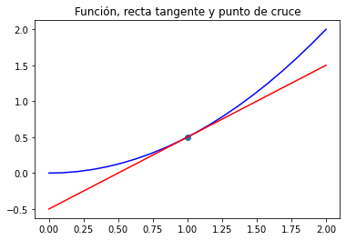
Recta tangente a una función#
La recta tangente a la función \(f(x)\) en \(x = x_0\) es la linea que pasa a través del punto \((x_0, f(x_0))\) y tiene la misma pendiente que la función en ese punto. La recta tangente a la función \(f(x)\) en el punto \(x = x_0\) está descrita por la ecuación $\(T_1(x) = f(x_0) + f'(x_0)(x − x_0)\)$
¿Cuál es la ecuación de la recta tangente a \(f(x) = \frac{1}{2}x^2\) en \(x_0 = 1\)?
# Crear las variables
x, f = symbols("x f")
# Crear la función
f = 1./2*x**2
print ('f(x)\t=', f)
f(x) = 0.5*x**2
# Encontrar la derivada
df = diff(f,x)
print ("f'(x)\t=", df)
f'(x) = 1.0*x
# Encontrar la recta tangente a la función
x0 = 1
T_1 = f.subs({x:x0}) + df.subs({x:x0}) * (x - x0)
print ("T1(x)\t=", T_1)
T1(x) = 1.0*x - 0.5
# Comprobar que el valor en el eje "y" de la función y la recta tangente son iguales
print(f.subs({x:1}))
T_1.subs({x:1})- f.subs({x:1})
0.500000000000000

# Comprobar que el valor de la pendiente de la función y la recta tangente son iguales
print(diff(f,x).subs({x:1}))
diff(T_1,x).subs({x:1}) - diff(f,x).subs({x:1})
1.00000000000000
# Obtener funciones de Python a partir de expresiones
fp = lambdify(x, f,   "numpy")
tp = lambdify(x, T_1, "numpy")
# Graficar
xr = np.linspace(0,2,20)
plt.plot(xr, fp(xr), color="blue") # función
plt.plot(xr, tp(xr), color="red")  # recta tangente
plt.scatter(x0, fp(x0)) #punto de cruce, x0 == 1
plt.title("Función, recta tangente y punto de cruce")
Text(0.5, 1.0, 'Función, recta tangente y punto de cruce')
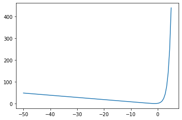
Ecuaciones diferenciales#
Resolver \(\frac{dy}{dt}=y(t)+t\)
# Crear variables
t, C1 = symbols("t C1")

# Crear una función no definida con el parámetro cls=Function
y = symbols("y", cls=Function)

# Crear una expresión con la función no definida y la variable
dydt = y(t)+t

# Crear la ecuación a resolver
eq = dydt-diff(y(t),t)
eq

# Resolver. Con dsolve se resuelven ecuaciones diferenciales
yt = dsolve(eq, y(t))
yt

# Obtener el resultado
yt.rhs

# Verificar la solución, forma 1
simplify(dydt.subs({y(t): yt.rhs}) - diff(yt.rhs,t))
# Verificar la solución, forma 2
expr1 = dydt.subs({y(t): yt.rhs})
expr2 = diff(yt.rhs,t)

expr1.equals(expr2)
True
# Usando condición inicial y(0) = 2, obtener C1
eq1 = Eq(yt.rhs.subs({t:0}).evalf(), 2.) # Eq(f,g) -> f=g
sol = solve([eq1], [C1])
sol

# Definir función para C1=3, con la variable "t"
C1_val = 3
fY = lambdify(t, yt.rhs.subs({C1: C1_val}), "numpy") # C1_val == 3
print(yt.rhs.subs({C1: C1_val}))

# Evaluar en un sólo valor de tiempo
print(fY(0))

# Evaluar en varios valores de tiempo y graficar
t_vals = np.linspace(-50,5,100)
plt.figure()
plt.plot(t_vals, fY(t_vals))
plt.show()
((-t - 1)*exp(-t) + 3)*exp(t)
2.0
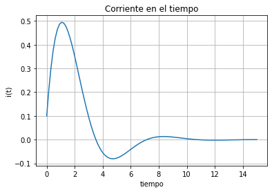
Circuito RLC#
Modelo:
\(\begin{array}{l} \frac{{di}}{{dt}} = - \frac{R}{L}i(t) - \frac{1}{L}v(t) + \frac{1}{L}vi\\ \frac{{dv}}{{dt}} = \frac{1}{C}i(t) \end{array}\)

# Definir simbolos y funciones
t, vi, L, R, C = symbols("t vi L R C")
C1,C2 = symbols("C1 C2")
v = Function("v")(t)
i = Function("i")(t)
didt=i.diff(t)
dvdt=v.diff(t)
# Primera expresión
expr1 = Eq(didt, (1/L)*vi-(R/L)*i-(1/L)*v)
expr1

# Segunda expresión
expr2 = Eq(dvdt, (1/C)*i)
expr2

# Sustitución, suponiendo valores conocidos
expr1=expr1.subs(L, 1).subs(R,1).subs(C,1).subs(vi,1)
expr1

# Sustitución, suponiendo valores conocidos
expr2=expr2.subs(C,1)
expr2

# Resolver usando dsolve. Se encontrará i(t) y v(t)
s=dsolve([expr1,expr2])
s

# Sustituir para un i(0)=0.1 y v(0)=0.1
eq1 = Eq(s[0].rhs.subs({t:0}).evalf(), 0.1) #i corriente
print(eq1)
eq2 = Eq(s[1].rhs.subs({t:0}).evalf(), 0.1) #v voltaje
print(eq2)
sol = solve([eq1,eq2], [C1,C2])
sol
Eq(-0.5*C1 - 0.866025403784439*C2, 0.1)
Eq(C1 + 1.0, 0.1)

# Ecuación corriente
e1 = lambdify(t,s[0].rhs.subs(sol),'numpy')
# Ecuación voltaje
e2 = lambdify(t,s[1].rhs.subs(sol),'numpy')
# Vector de valores en el tiempo
t_vals = np.linspace(0,15,100)

# Graficar
plt.figure()
plt.plot(t_vals, e1(t_vals))
plt.xlabel('tiempo')
plt.ylabel('i(t)')
plt.grid(True)
plt.title("Corriente en el tiempo")
plt.show()
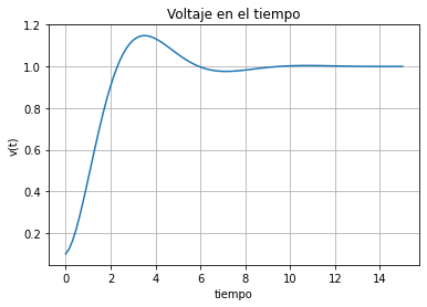
# Graficar
plt.plot(t_vals, e2(t_vals))
plt.xlabel('tiempo')
plt.ylabel('v(t)')
plt.grid(True)
plt.title("Voltaje en el tiempo")
plt.show()
Oscilador armónico amortiguado#
# Crear la ecuación del oscilador
t, w = symbols("t \\omega_0", positive=True)
d = symbols("\\xi", real=True)
x = Function("x", real=True)
eq = w**2*x(t) + 2*w*d*x(t).diff(t) + x(t).diff(t,t)
eq

Evaluar y resolver para cuando \(\omega=0\) y \(\xi=1/10\)
# Evaluar para las condiciones iniciales
eq = eq.subs(w, 1).subs(d, Rational(1,10))

# Resolver la ecuación diferencial
sol = dsolve(eq,x(t))
sol

# Usando estas condiciones iniciales x(0) = 1, y para dx(0)/dt = 0
C1, C2 = symbols("C1, C2")
const = solve([sol.rhs.subs(t,0) - 1, sol.rhs.diff(t).subs(t, 0)], [C1,C2])
print ("const =", const)

# Reemplazar C1 y C2 en la solución
initvalue_solution = sol.rhs.subs(C1, const[C1]).subs(C2, const[C2])
print ("Aplicando las condiciones iniciales \nx(t) = ")
initvalue_solution
const = {C1: sqrt(11)/33, C2: 1}
Aplicando las condiciones iniciales
x(t) =

# Graficar
T = np.linspace(0, 10)
F = lambdify(t, initvalue_solution, "numpy")
dFdT = lambdify(t, initvalue_solution.diff(), "numpy")
plt.plot(T, F(T))
plt.plot(T, dFdT(T))
plt.legend(("f(t)", "df(t)/dt"))
plt.xlabel("t")
plt.show()
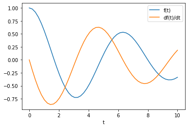
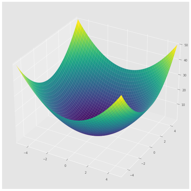
Gráfico en 3D#
from sympy import symbols
from sympy.plotting import plot3d
x, y = symbols('x y')
plot3d(x**2+y**2, (x, -5, 5), (y, -5, 5))
<sympy.plotting.plot.Plot at 0x7f0ced2dd760>
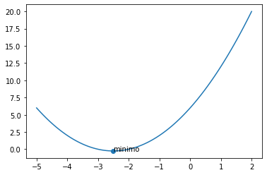
Calculo del mínimo en una variable de forma analítica#
x,y =symbols("x,y")
y=x**2+5*x+6
fp = lambdify(x, y,   "numpy")
y

df=diff(y)
df

pc=solve(df)
N(pc[0])

d2f=diff(df)
d2f

cy=y.subs({x:N(pc[0])})
cy

z=np.linspace(-5,2,100)
plt.plot(z,fp(z))
plt.scatter(pc[0],fp(pc[0]))
plt.text(pc[0],fp(pc[0]),'minimo')
Text(-5/2, -1/4, 'minimo')
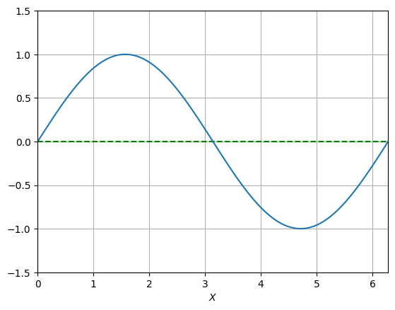
Graficas dinámicas#
# Librerias necesarias para realizar el gráfico
import numpy as np
import matplotlib.pylab as plt
from matplotlib import animation, rc
from IPython.display import HTML;
rc('animation', html='html5');
# Plantilla sobre la cual se realiza el gráfico
x = np.linspace(0, 2 * np.pi, 100)
y = np.sin(x)

fig, ax = plt.subplots()
ax.set_xlabel('$X$')
ax.set_xlim(0, 2 * np.pi)
ax.set_ylim(-1.5, 1.5)
ax.grid(True)
plt.plot([0,2*np.pi], [0, 0], '--', color='green')
plt.plot(x,y)

# Se definen los atributos que debe tener la linea o en este caso el punto que se va a pintar en cada iteracion
linea, = ax.plot([],[],'o',color = 'r', label = 'Curva sin(x)')
# Realizamos una función que grafique el punto especifico uno a uno

frames = 100;
def graficar(i):

  x = np.linspace(0, 2 * np.pi, 100)
  y = np.sin(x)

  linea.set_data(x[i],y[i])
  return (linea,)
# Ejecutamos la animación para que se genere y quede en loop mostrando su resultado.
anim = animation.FuncAnimation(fig, graficar, frames=frames, interval=100)
anim
<ipython-input-56-d6bd03730612>:7: MatplotlibDeprecationWarning: Setting data with a non sequence type is deprecated since 3.7 and will be remove two minor releases later
  linea.set_data(x[i],y[i])
Enlace de interés para animación:
Plotly#
Plotly es un framework interactivo de visualización de datos ampliamente utilizado por su capacidad para crear gráficos interactivos y elegantes. Con una sintaxis sencilla y versatilidad, Plotly permite a los usuarios crear visualizaciones atractivas que responden a la interacción del usuario, como gráficos de dispersión, barras, líneas y más. Su popularidad radica en su capacidad para producir gráficos dinámicos y personalizables en aplicaciones web, informes y paneles de control. Ya sea para analizar datos, comunicar ideas de manera efectiva o explorar patrones, Plotly brinda una herramienta poderosa y flexible para la creación de visualizaciones de datos interactivas y atractivas.
# Instalemos la librería
!pip install plotly
Requirement already satisfied: plotly in /usr/local/lib/python3.10/dist-packages (5.13.1)
Requirement already satisfied: tenacity>=6.2.0 in /usr/local/lib/python3.10/dist-packages (from plotly) (8.2.2)
import plotly.express as px
df = px.data.iris()
fig = px.scatter(df, x="sepal_width", y="sepal_length", color="species",
                 size='petal_length', hover_data=['petal_width'])
fig.show()
import plotly.express as px

# Datos de ejemplo
labels = ['Manzanas', 'Plátanos', 'Uvas', 'Naranjas']
values = [30, 25, 20, 15]

# Crear el gráfico de torta
fig = px.pie(names=labels, values=values, title='Gráfico de Torta')

# Mostrar el gráfico
fig.show()
import plotly.graph_objs as go

# Crear una malla de puntos en el dominio deseado
x_vals = y_vals = list(range(-5, 6))
x_grid, y_grid = np.meshgrid(x_vals, y_vals)

# Calcular los valores de z utilizando la función
z_vals = x_grid**2 + y_grid**2

# Crear la figura 3D
fig = go.Figure(data=[go.Surface(z=z_vals, x=x_grid, y=y_grid)])

# Configurar el título y los nombres de los ejes
fig.update_layout(title='Gráfico 3D de x^2 + y^2', scene=dict(xaxis_title='X', yaxis_title='Y', zaxis_title='Z'))

# Mostrar la figura
fig.show()
import numpy as np
import plotly.graph_objs as go
from plotly.subplots import make_subplots

# Crear una malla de puntos en el dominio deseado
x_vals = y_vals = list(range(-5, 6))
x_grid, y_grid = np.meshgrid(x_vals, y_vals)

# Calcular los valores de z utilizando la función
z_vals = x_grid**2 + y_grid**2

# Crear la figura 3D y un subplot para los sliders
fig = make_subplots(rows=1, cols=2, specs=[[{'type': 'surface'}, {'type': 'xy'}]])

# Agregar la superficie al subplot izquierdo
surface = go.Surface(z=z_vals, x=x_grid, y=y_grid)
fig.add_trace(surface, row=1, col=1)

# Agregar un punto en (0, 0, 0)
point = go.Scatter3d(x=[0], y=[0], z=[0], mode='markers', marker=dict(size=10, color='red'))
fig.add_trace(point, row=1, col=1)

# Configurar el diseño de la figura
fig.update_layout(
    scene=dict(xaxis_title='X', yaxis_title='Y', zaxis_title='Z'),
    scene_aspectmode='cube'
)

# Mostrar la figura
fig.show()
import plotly.graph_objects as go
import numpy as np

# Create figure
fig = go.Figure()

# Add traces, one for each slider step
for step in np.arange(0, 5, 0.1):
    fig.add_trace(
        go.Scatter(
            visible=False,
            line=dict(color="#00CED1", width=6),
            name="𝜈 = " + str(step),
            x=np.arange(0, 10, 0.01),
            y=np.sin(step * np.arange(0, 10, 0.01))))

# Make 10th trace visible
fig.data[10].visible = True

# Create and add slider
steps = []
for i in range(len(fig.data)):
    step = dict(
        method="update",
        args=[{"visible": [False] * len(fig.data)},
              {"title": "Slider switched to step: " + str(i)}],  # layout attribute
    )
    step["args"][0]["visible"][i] = True  # Toggle i'th trace to "visible"
    steps.append(step)

sliders = [dict(
    active=10,
    currentvalue={"prefix": "Frequency: "},
    pad={"t": 50},
    steps=steps
)]

fig.update_layout(
    sliders=sliders
)

fig.show()